4. Monitoring LAMMPS output

4.1. Output Window

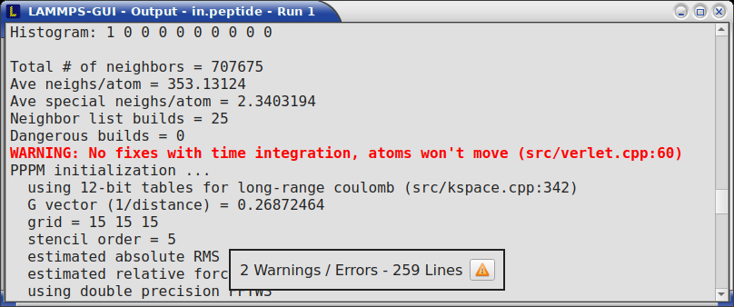
By default, when starting a run, an Output window opens that displays the screen output of the running LAMMPS calculation, as shown below. This text would normally be seen in the command-line window.

LAMMPS-GUI captures the screen output from LAMMPS as it is generated and updates the Output window regularly during a run. If there are any warnings or errors in the LAMMPS output, they are highlighted by using bold text colored in red. There is a small panel at the bottom center of the Output window showing how many warnings and errors were detected and how many lines the entire output has. By clicking on the button on the right with the warning symbol or by using the keyboard shortcut Ctrl-N (Command-N on macOS), you can jump to the next line with a warning or error. If there is a URL pointing to additional explanations in the online manual, that URL will be highlighted and double-clicking on it shall open the corresponding manual page in the web browser. The option is also available from the context menu.

By default, the Output window is replaced each time a run is started. The runs are counted and the run number for the current run is displayed in the window title. It is possible to change the behavior of LAMMPS-GUI in the preferences dialog to create a new Output window for every run or to not show the current Output window. It is also possible to show or hide the current Output window from the View menu.

The text in the Output window is read-only and cannot be modified, but keyboard shortcuts to select and copy all or parts of the text can be used to transfer text to another program. Also, the keyboard shortcut Ctrl-S (Command-S on macOS) is available to save the Output buffer to a file. The “Select All” and “Copy” functions, as well as a “Save Log to File” option are also available from a context menu by clicking with the right mouse button into the Output window text area.

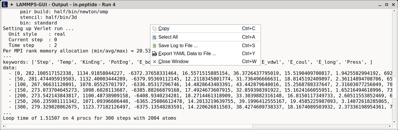
Should the Output window contain embedded YAML format text (see above for a demonstration), for example from using thermo_style yaml or thermo_modify line yaml, the keyboard shortcut Ctrl-Y (Command-Y on macOS) is available to save only the YAML parts to a file. This option is also available from a context menu by clicking with the right mouse button into the Output window text area.

4.2. Charts Window

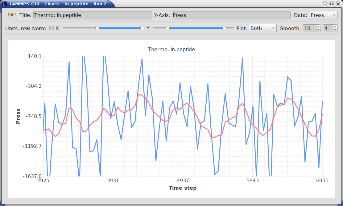
By default, when starting a run, a Charts window opens that displays a plot of thermodynamic output of the LAMMPS calculation as shown below.

The “Data:” drop down menu on the top right allows selection of different properties that are computed and written as thermodynamic output to the output window. Only one property can be shown at a time. The plots are updated regularly with new data as the run progresses, so they can be used to visually monitor the evolution of available properties. The update interval can be set in the Preferences dialog. By default, the raw data for the selected property is plotted as a blue graph. From the “Plot:” drop menu on the second row (immediately to the right of the Chart Style… and Postprocess… quick-access buttons), you can select whether to plot only raw data graph, only a smoothed data graph, or both graphs on top of each other. The smoothing process uses a Savitzky-Golay convolution filter. The convolution window width (left) and order (right) parameters can be set in the boxes next to the drop down menu. Default settings are 10 and 4 which means that the smoothing window includes 10 points each to the left and the right of the current data point for a total of 21 points and a fourth order polynomial is fitted to the data in the window.

The “Title:” and “Y:” input boxes allow to edit the text shown as the plot title and the y-axis label, respectively. The text entered in the “Title:” box is applied to all charts, while the “Y:” text changes only the y-axis label of the currently selected plot. In standalone plot mode (when plotting an external data file), an additional “X-Axis:” input box is shown to the right of “Y:” and sets the x-axis label for all charts.

The window title shows the current run number that this chart window corresponds to. Same as for the Output window, the chart window is replaced on each new run, but the behavior can be changed in the Preferences dialog.

From the File menu on the top left, it is possible to save an image of the currently displayed plot or export the data in either plain text columns (for use by plotting tools like gnuplot or grace), as CSV data which can be imported for further processing with Microsoft Excel, LibreOffice Calc, or with Python via pandas, or as YAML which can be imported into Python with PyYAML or pandas.

Thermo output data from successive run commands in the input script is combined into a single data set unless the format, number, or names of output columns are changed with a thermo_style or a thermo_modify command, or the current time step is reset with reset_timestep, or if a clear command is issued. This is where the YAML export from the Charts window differs from that of the Output window: here you get the compounded data set starting with the last change of output fields or timestep setting, while the export from the log will contain all YAML output but segmented into individual runs.

Adjusting the chart style. The Chart Style… entry in the chart window’s File menu, or the chart-style quick-access button at the far left of the second toolbar row, opens a dialog to change how the data is drawn. The Raw data and Processed data series each have independent settings for the display style (Lines, Points, or Lines and Points), the color, the line width, and the point size. This makes it possible, for example, to show the raw data as faint points and the smoothed curve as a bold line. The Legend placement selector in the same dialog adds an in-plot legend that lists the visible named series; it can be turned Off or anchored to any of the four plot corners (Top left, Top right, Bottom right, or Bottom left). The selected placement is remembered across sessions.

Added in version 2.1: The Chart Style dialog and the independent styling of the raw and processed series were added, including the per-series point size and the optional in-plot legend.

Reference lines. The Reference Lines… entry in the chart window’s File menu opens a dialog for adding straight annotation lines that are drawn on every chart in the window. Each line is either Vertical (at a chosen x value) or Horizontal (at a chosen y value) and can carry a text label and an individually chosen color. The label position along the line (Top, Center, or Bottom for vertical lines; Left, Center, or Right for horizontal lines) is selected per line, while the label font size, the gap between the label and the line, and whether the labels are drawn in an opaque box apply to the whole window. Reference lines are useful, for example, to mark a target temperature, a transition point, or a fitted value.

Added in version 2.1: The Reference Lines dialog was added.

Post-processing the data. The Postprocess… entry in the chart window’s File menu, or the quick-access button immediately to the right of the Chart Style… button, runs an analysis on the data of the currently selected property. The following analyses are available:

• Autocorrelation computes the normalized autocorrelation function of the selected data up to a chosen maximum lag and shows it in a new chart window (the abscissa becomes the lag). This is useful, for example, for estimating correlation times of fluctuating quantities.

• Polynomial fit performs a least-squares fit of a polynomial of a chosen degree, overlays the fitted curve on the chart, and reports the coefficients and the root-mean-square residual.

• Birch-Murnaghan EOS fit fits a 4-parameter Birch-Murnaghan equation of state to energy-versus-volume data (x = volume per unit cell, y = energy). A confirmation dialog lets you verify the x and y column assignments and enter the number of atoms in the conventional unit cell N (default 1; e.g. 4 for FCC, 2 for BCC or HCP; use N = 1 when the x data is already the conventional cell volume rather than volume per atom). The fit reports the equilibrium volume V₀, the derived lattice constant a₀ = (N V₀)^1/3, the equilibrium energy E₀, the bulk modulus B₀, and its pressure derivative B₀’.

• Custom function evaluates a user-supplied mathematical expression f(x) over the x range of the data and overlays it as a curve. The expression uses the variable x for the abscissa and supports the usual arithmetic operators and functions (for example 2*x^2 + 3*sin(x)).

• Custom fit performs a nonlinear least-squares fit of a user-supplied expression to the data. In addition to the expression, you provide the fit parameters and their initial guesses as name=value pairs (for example a=1, b=0.5) and, optionally, a label for the fitted curve. The fit uses a Levenberg-Marquardt algorithm with analytic derivatives of the expression; on success the fitted curve is overlaid and the fitted parameters, the root-mean-square residual, and the number of iterations are reported.

The expressions for Custom function and Custom fit are parsed and evaluated with a bundled subset of the Lepton expression parser, the same library used by the LAMMPS Lepton-based styles, so the supported syntax matches.

When any fit or custom-function overlay is active, the “Plot:” drop-down treats the overlay as the “smoothed” series: selecting “Smoothed” or “Both” shows the overlay curve, while selecting “Raw” hides it. This applies uniformly to all analysis types (polynomial, EOS, custom function, and custom fit).

Added in version 2.1: The Postprocess dialog with the autocorrelation, polynomial, Birch-Murnaghan EOS, custom-function, and custom-fit analyses was added.

The same Charts window is also used to plot data from an external file opened with File -> Plot Data File… (Ctrl-Shift-P, see the File menu); in that standalone mode there is no associated simulation, so the Units and Norm controls are hidden. The column-picker dialog shown before the chart opens lets you select which column provides the x axis and which columns to plot, and also allows renaming columns. An “X-Axis:” label field in the first toolbar row (to the right of “Title:” and “Y:”) lets you edit the x-axis label after the chart opens. All the styling, export, and post-processing features described above work the same way. The same column-picker and standalone chart window are also launched when LAMMPS-GUI is invoked from the command line with the -c/--chart flag (see command-line options).

The Preferences dialog has a Charts tab, where you can configure multiple chart-related settings, like the default title, colors for the graphs, default choice of the raw / smooth graph selection, whether the grid for the major and minor ticks is drawn, and the default chart graph size.

Slowdown of Simulations from Charts Data Processing

Using frequent thermo output during long simulations can result in a significant slowdown of that simulation since it is accumulating many data points for each of the thermo properties in the chart window to be redrawn with every update. The updates are consuming additional CPU time when smoothing enabled. This slowdown can be confirmed when an increasing percentage of the total run time is spent in the “Output” or “Other” sections of the MPI task timing breakdown. It is thus recommended to use a large enough value as argument N for the thermo command and to select plotting only the “Raw” data in the Charts Window during such simulations. It is always possible to switch between the different display styles for charts during the simulation and after it has finished.

Changed in version 1.7: As of LAMMPS-GUI version 1.7 the chart data processing is significantly optimized compared to older versions of LAMMPS-GUI. The general problem of accumulating excessive amounts of data and the overhead of too frequently polling LAMMPS for new data cannot be optimized away, though. If necessary, the command line LAMMPS executable needs to be used and the output accumulated on a very fast disk (e.g. a high-performance SSD).

4.3. Variable Info

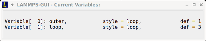
During a run, it may be of interest to monitor the value of input script variables, for example to monitor the progress of loops. This can be done by enabling the “Variables Window” in the View menu or by using the Ctrl-Shift-W keyboard shortcut. This shows info similar to the info variables command in a separate window as shown below.

Like for the Output and Charts windows, its content is continuously updated during a run. It will show “(none)” if there are no variables defined. Note that it is also possible to set index style variables, that would normally be set via command-line flags, via the “Set Variables…” dialog from the Run menu. LAMMPS-GUI automatically defines the variable “gui_run” to the current value of the run counter. That way it is possible to automatically record a separate log for each run attempt by using the command

log logfile-${gui_run}.txt

at the beginning of an input file. That would record logs to files logfile-1.txt, logfile-2.txt, and so on for successive runs.